UzK Operations Management Course Summary

A summary for the Operations Management course at the University of Cologne in the summer semester of 2017.

This course was separated into two parts. Supply Chain Operations and Behavioral Economics. They were taught by Prof. Thonemann and Prof. Becker-Peth. Most of the graphics are taken from the slide decks of these two professors.

Supply Chain Operations

Motivational Reasons for Supply Chain Management

Bullwhip effect

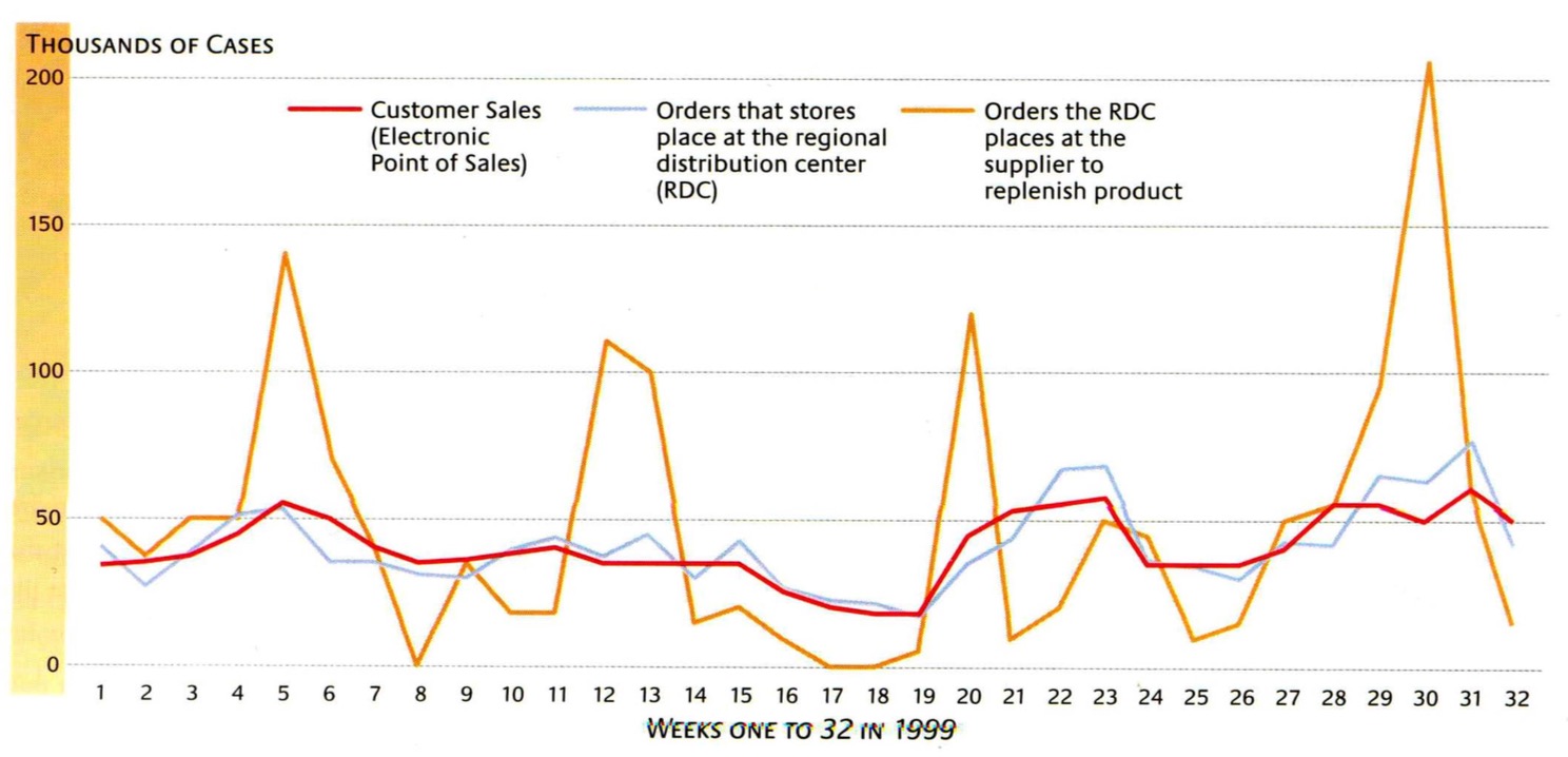
The Bullwhip effect describes a phenomenon where small fluctuations in the end-customer demand lead to ever-increasing fluctuations of the demand down the supply chain. This is mainly caused by overreaction of individual supply chain participants to small fluctuations in demand.

The effect can be mediated by automated sharing of demand data across the supply chain. However, this is often not implemented due to business reasons. An example would be the non-disclosed amount of Apple watch sales. An alternative is the use of contracts to ensure a minimum and maximum demand per period with additional demand being offered at a higher premium.

Causes:

• inadequate information sharing
• lead time and delay of shipments vs. incoming orders
• loss aversion, overreaction
• periodic review inventory model leads to aggregation of orders to large sums

Bullwhip factor

$$ BF(LT,T) \approx 1 + \frac{2(LT+1)}{T}+ \frac{2(LT+1)^ 2}{T ^2} \mid LT:\text{lead time}, T:\text{forecasting error periods} $$

Newsvendor Model

Facts (Reproduction)

• placing orders before demand is known
• overage and underage costs apply
  • overage → $w-bb$ or $w-v$ (buyback / salavage)
  • underage → lost sale opportunities

Formulas (Application)

variable	description
$c_o, c_u$	overage cost, underage cost
$p_y$	probability that demand will be y
$c$	unit order cost
$S$	order Quantity

Critical Ratio $$F(S)=\frac{c_u}{c_u+c_o}=CR$$

Optimal order quantity $$S^* = F^{-1}\left(\frac{c_u}{c_u+c_o}\right)$$ **In case of normally distributed demand** $$S^* = \mu + z\sigma \mid z=F^{-1}\left(\frac{c_u}{c_u+c_o}\right)$$

Optimal expected cost

$$ Z(S^ * ) = (c_u+c_o)\cdot f_{N(0,1)}(z) \cdot \sigma $$ **Optimal expected profit** $$ \Pi(S^* ) = (r-c)\mu-Z(S^ * ) $$

Formulas (Application)

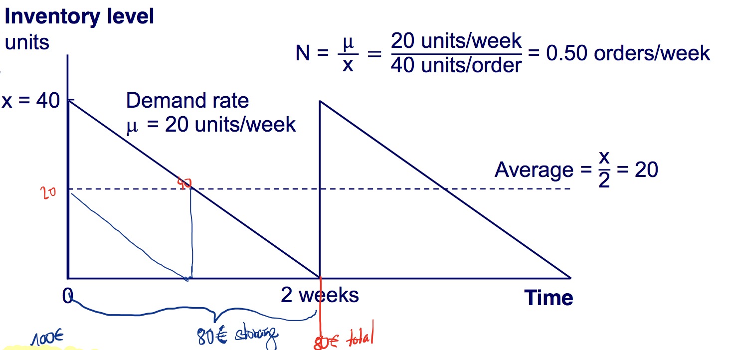
Economic Order Quantity Model

Facts (Reproduction)

• assumes a constant demand
• orders arrive instantly
• fixed order costs and linearly dependent storage costs
• approach is: large fixed order costs increase order quantity, large holding costs decrease the number

Formulas (Application)

variable	description
$\mu$	demand rate p period
$K$	fixed order cost
$c$	variable order cost(unit/order)
$h$	inventory holding cost (unit/period)
$x$	order quantity

optimal order quantity $$ x^* = \sqrt{\frac{2K\mu}{h}} $$

total cost per period inventory holding cost + fixed order cost + variable order cost $$Z(x) = h\frac{x}{2} + K\frac{\mu}{x} + c\mu$$

Facts (Reproduction)

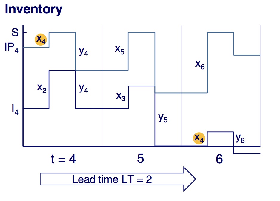
• orders arrive after lead time
• excess demand is back-ordered
• at each period order the difference between the current inventory positions (inventory - outstanding orders) and the order-up-to inventory level S

Process of each session is:

1. Observe inventory level $I_t$
2. Observe open orders $O_t$
3. Compute inventory position $IP_t$
4. Place order $x_t = S– IP_t$
5. Receive shipment $x_{t-LT}$
6. Fill demand $y_t$

Formulas (Application)

variable	description
$f(y)$	Density function of demand y
$F(y)$	Distribution function of demand y
$c$	Unit cost (0.50 €/unit)
$h$	Unit inventory holding cost
$p$	Unit backorder penalty cost
$r$	Unit revenue
$LT$	Lead time
$a$	almost b

Optimal order-up-to level As in the other cases, we use the standard formula $\mu+z\sigma$ with the parameter of this model as seen below $$ S^* = \mu +z\sigma_ {LT+1} \mid z = F_ {LT+1}^{-1}\left(\frac{p}{p+h}\right) $$

To calculate LT+1 is used

$$ \sigma_{LT+R} = \sigma \sqrt{LT+R} \mid R=\text{review period}$$

To calculate expected costs of optimal solution

$$ Z(S^* ) = (h+p)\cdot f_{N(0,1)}(z)\cdot \sigma_{LT+1}$$

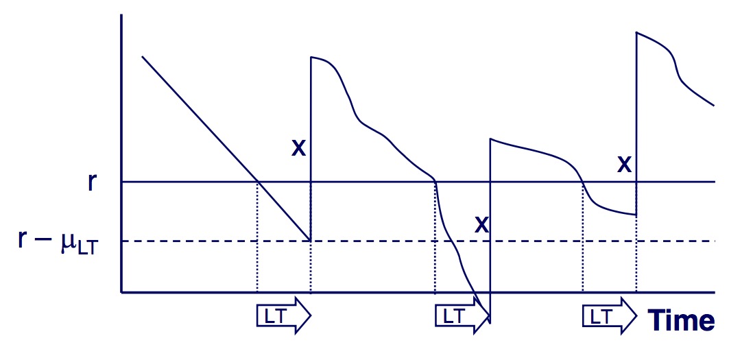
Continuous Review Inventory Model

Facts (Reproduction)

Formulas (Application)

variable	description
$\mu$	mean demand
$\sigma$	standard deviation of demand
$h$	inventory holding cost
$p$	unit backorder penalty
$K$	fixed order cost
$LT$	lead time
$r$	reorder point (number not time)
$x$	order quantity (often also $q$)

expected inventory $$ E[\text{inventory}]\approx r-\sigma_{LT} + \frac{x}{2} $$

Expected costs Here, the first describes the holding cost, the second term the expected penalty cost and the third the order cost/period.

$$ Z(x,r) \approx h \left(r-\mu_{LT}+\frac{x}{2}\right)+ p\frac{\mu}{x}L\left(\frac{r-\mu_{LT}}{\sigma_{LT}}\right)+ K \frac{\mu}{x} $$

Service Levels

• $\alpha$-service level: probability that all demand in an order cycle is met must be at least $\alpha$
  • to calculate the alpha service level, we need to look at the reorder point. If the reorder point is below the expected demand for the lead time plus a safety factor (which is dependent on the ɑ-level), we need to reorder. The reorder amount can still be determined using the iterative solution
• $\beta$-service level: expected fraction that is filled in an order cycle must be at least $\beta$
  • the β-service level calculations are similar to those of the ɑ. The reorder amount is again determined by the approaches of the continuous review model. The reorder point is similar as with ɑ-level, however we use the inverse loss function instead and the parameter is dependent on $\sigma$ and $x^*$.

Formulas (Application)

ɑ-Service level

Optimal order quantity

$$x^* = \sqrt{\frac{2\mu K}{h}}$$

Optimal reorder point

$$r^* = F_{LT}^{-1}(\alpha) = \mu_ {LT}+z\sigma_{LT}$$

β-Service level

Optimal order quantity is the same as with ɑ-Service

Optimal reorder point

$$ r^* = \mu_{LT} + L^{-1}\left(\frac{(1-\beta)\mu }{\sigma_ {LT}}\right) \sigma_{LT} $$

$$ \beta \approx \frac{\mu-L\left(\frac{S^* - \mu_{LT+1}}{\sigma_{LT+1}}\right)}{\mu} $$

Expected backorder levels $$ E(O-S) ^+=\sum_{y=S} ^{\infty}(y-S)p_y $$

Demand Estimation

Facts (Reproduction)

• demand estimation, also called forecasting
• target service level and expected demand lead to order quantity and reorder point adaptation

Generally there are two approaches

1. Distribution parameter fitting (i.e. figuring out the underlying function of the demand distribution)
2. Demand forecasting
   • moving averages
   • double exponential smoothing
     • the standard deviation for the forecast is not based on the past deviations but instead on the forecast error. The better the forecasts were in the past few phases, the more narrow is our estimation variance for the upcoming periods.

Formulas (Application)

variable	description
$\hat{y_t}$	forecasting for period t
$\epsilon_t$	forecast error ($e_t^2$ for squared err)
$M$	number of data points for forecast error
$N$	Degrees of freedom (1 for moving average, 2 for DES)

exponential smoothing

standard deviation of demand

$$ \hat{\mu}_ t = \sqrt{\frac{1}{M-N} \sum_ {k=t-M} ^{t-1}{\epsilon_k ^2}} $$

Revenue Management

Finding the right price for different products with limited availability.

• Overbooking
• Discount allocation (e.g. nested policies and protection levels)
• traffic management

Fencing

• Parameters used for fencing tactics are: Time, Location, Flexibility, Groups, Variants

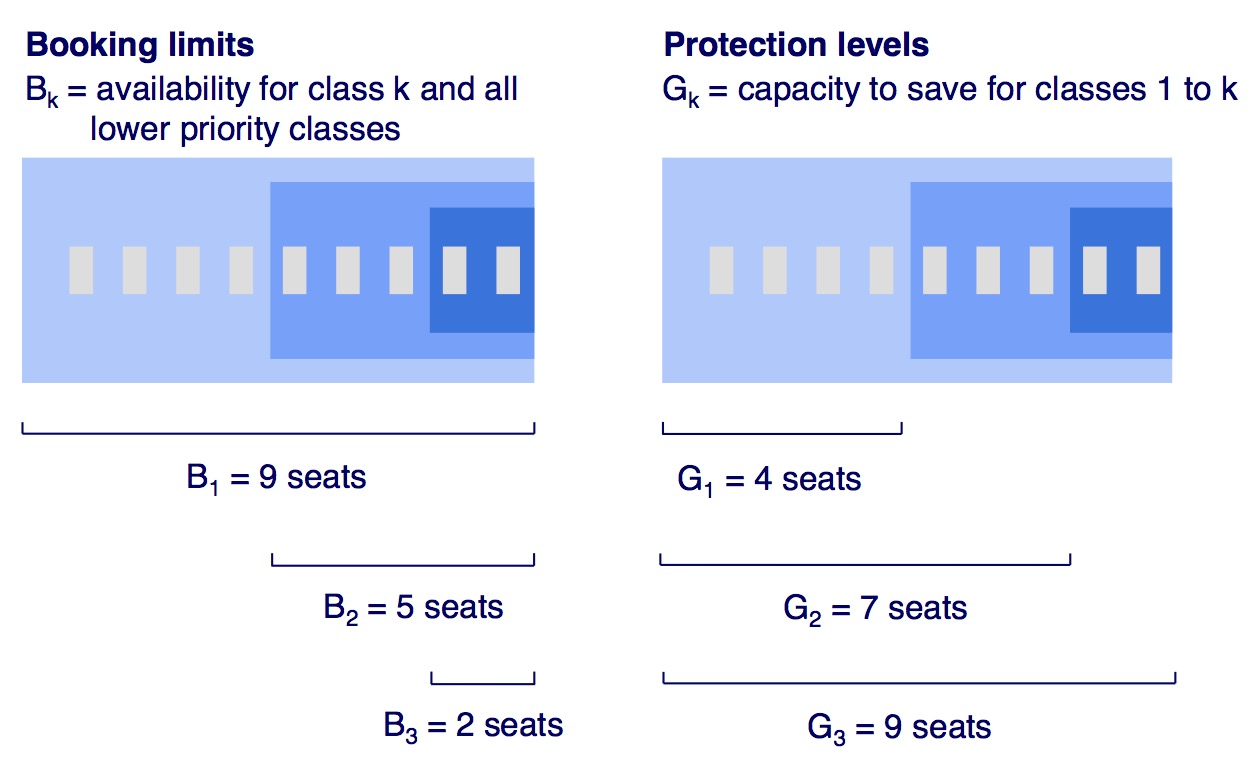
• with booking limits, if there are 10 spots available and 3 are allocated for the cheapest tier, once 3 bookings occur, independent of category, the lowest class is booked out.
• Protection Level: minimum amount of seats reserved for certain class
• Booking Limit: Max amount of bookings possible for a class

Littlewood’s Rule - Optimizing reservations

• Assumption: low-price customers book before high-price customers
• demand distribution of high-price customers is known
• low-price demand exceeds capacity

Approach: Set reserved amount for high priced booking class to 0. Now iterate over the possible number of reserved spots and calculate expected revenue. Once revenue doesn’t improve anymore, stop.

Calculating protection levels for 2 classes

variable	description
$C$	capacity
$r_i$	revenue for class i
$B_i$	bookings for class i
$G_i$	protection level for class i

$$ G_1^* = C-B_2^* = F_1^{-1}\left(1-\frac{r_2}{r_1}\right) $$

This approach can obviously also be used for several classes. For each class, the previous classes need to be solved first. So with four classes high – medium – low – trash, first we calculate the protection amount for the high class, then for the medium etc. until we have a set of nested protection amounts for each class.

Protection levels for n classes

1. Calculate protection levels for each class against k+1 class $$ G_{k+1,I} = F_1^{-1}\left(1-\frac{r_{k+1}}{r_I}\right) $$
2. Aggregate protection levels for each class: Protection level of high class is sum of all protection levels in the classes below.
3. Calculate booking limits $$ B_k = C - G_{k-1} $$

This approach can obviously also be used for several classes. For each class, the previous classes need to be solved first. So with four classes high – medium – low – trash, first we calculate the protection amount for the high class, then for the medium etc. until we have a set of nested protection amounts for each class.

Protection levels for n classes

1. Calculate protection levels for each class against k+1 class $$ G_{k+1,I} = F_1^{-1}\left(1-\frac{r_{k+1}}{r_I}\right) $$
2. Aggregate protection levels for each class: Protection level of high class is sum of all protection levels in the classes below.
3. Calculate booking limits $$ B_k = C - G_{k-1} $$

Overbooking

Calculation of overbooking amount

variable	description
$C$	capacity
$B$	booking limits
$r$	price of one unit sold
$p$	cost of paying for overbooked customer
$x$	number of no-shows
$y$	demand
$f(x)$	density function of no-shows

$$ B^* = C+F^{-1}\left(\frac{r}{p}\right) $$

and for ɸ-distributions

$$ B^* = C + \mu_ x + F_ {0,1}^{-1}\left(\frac{r}{p}\right)\sigma_ x $$

Markdown Management

Reducing prices for products that are nearing their end-of-life and will soon stop being sold. Solutions are suggested to be calculated using the Excel solver (which uses a simplex algorithm).

System approach

• The idea of looking at the supply chain as a network that enables systems to function
• if one part is missing, the whole product / system stands still (e.g. a plane)
• while service levels look at the number of missed orders and assume that customers then go and get the part somewhere else, the backorder-level looks at the number of days a system has to be put on hold until the business can supply the requested part. So customers “stay waiting” until they get their order.

Marginal Allocation Algorithm

If one has to stock several parts, which parts to stock and how many of each part for a given budget to minimize expected backorders

• $h(S)$ = expected backorder level
• $c_i$ = cost for part i

1.  Set $S_i = 0 \forall i=1,...,N$
2.  Compute marginal utility/cost change per part (i.e. one more of each => increase in costs)
    -   $m_i = \frac{h_i(S_i)-h_i(S_i+1)}{c_i} \forall i$
3.  Kick those out whose cost would go over budget
4. select $max\{m_i\}\forall i \in N$
5. Increase chosen max utility increasing $S_i$ by 1
6. if $\sum c_iS_i \leq b$ and not all kicked out jump to (3) else END

METRICs of cost analysis

• dependencies between parts (systems approach)
• Dependencies between echelons (expected delay at upper echelons because of backordering)

Strategic Safety Stock Placement in Multi-Echelon SC Networks

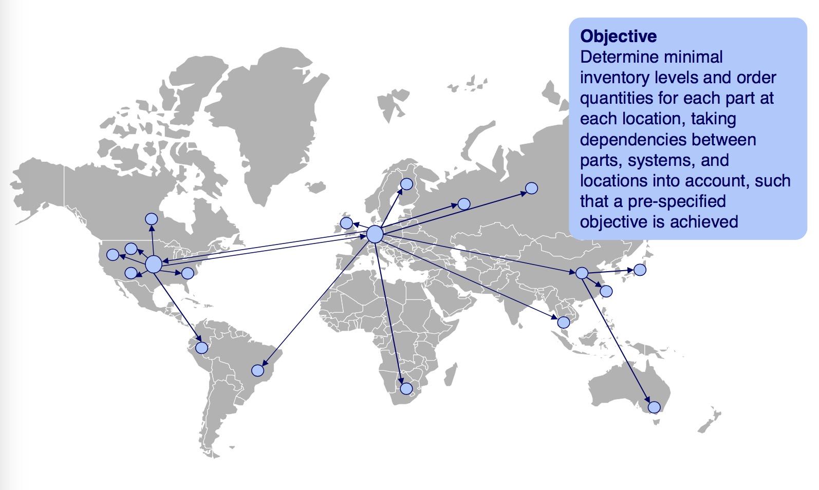
A big problem with a multi-tier production network is the large amount of decision variables that interact with each other and are interdependent, leading to a large and complex multidimensional problem with many constraints. One tries to find an optimal solution for the stock levels at each depot and the central warehouse to minimize overall costs while maintaining a certain service level.

Serial structures

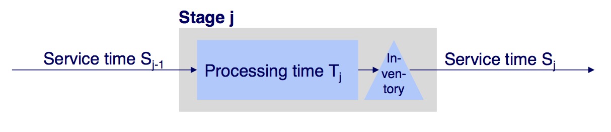
The overall idea is that each preceding stage has a promised service time. Stage j also promises its service time $S_j$ and while doing so tries to minimize its inventory

variable	description
$I_j(t)$	Inventory level at end of period t
$B_j$	Base-stock level of stage j
$d_j(a, b)$	Demand of periods $d_j(a)$ + … + $d_j(b)$
$S_{j-1}$	Inbound guaranteed service time
$S_j$	outbound guaranteed service time
$T_j$	Processing time of stage j

Observations:

• $\downarrow S_{j-1} \implies \downarrow B_j$
• $\uparrow d_j(a,b) \implies \uparrow B_j$
• $\uparrow T_j \implies \uparrow S_j$

Arbitrary structures

• Use of dynamic programming to solve complex systems

Supply Chain Management Case Studies

Inventory Management

TODO

HP

Current situation

• All production in one factory
• both standard steps and customization in globally delivering factory
• i18n’ized products shipped to different DCs in Asia, US and Europe
• especially europe suffering large product shortages for some markets while others were stockpiling
• large storage costs and at the same time low β-service level

possibel fixes

• short-term
  • Air shipments to quickly meet spikes in demand(expensive)
  • increase safety stocks for problematic product-market combinations
• long-term
  • DC localization
    • Move final assembly to DC, allowing Europe to use the generic shipments to serve all markets with only a few days of lag
  • european factory

HP optimization

• LT = 5 weeks (+1 review period)
• β-service level: 0.98
• buy: 400, sell: 600
• COC: 30% → 0.005357 / week

$$ r^* = \mu_ {LT} + L^{-1}\left(\frac{(1-\beta)\mu }{\sigma_ {LT}}\right) \sigma_ {LT} $$

$$ r^* = 31887 + L^{-1}\left(\frac{(1-0.98)31887 }{7335}\right) 7335 $$

$$ r^* = 31887 + 0.98 \cdot 7335 \approx 39075 $$

Barilla

Barilla was struggling with high variances in their retailer ordering patterns, a typical case of the bullwhip effect. Although the demand for pasta was largely constant with slight but clearly prognosable changes in certain seasons, the overall demand did not fluctuate. However, the three echelon supply chain caused Barilla to observe strong spikes of orders. Additionally, the sales team’s incentives were largely oriented towards overall sales volume and didn’t include avoidance of purchase spikes. Hence, sconti were given to the wholesalers, leading them to perform bulk purchases to make use of the cheaper rates.

Wholesalers expected quick deliveries but Barilla needed to follow a specific production plan to produce the different pasta types in good quality.

Solution approaches:

• JITD - just in time delivery
  • integration of inventory systems with Wholesalers
  • push instead of pull based ordering systems
  • promises: increased service levels and decreased storage costs for Barilla products
• Advanced forecasting: Barilla implemented a sophisticated demand forecast tool and was able to precisely predict demands for different markets and regions

Obermeyer

TODO

Behavioral Economics

Two systems of thinking

The human mind can be modeled as having two systems: The conscious, effortful system that is “single threaded” and requires our attention and the unconscious automatic and heuristics driven system that processes vast amounts of parallel streams of data but can hardly be controlled.

System 1: The conscious stream follows rules and can adapt to new tasks. It takes control force of will to continually focus on a certain topic without switching to other topics of interest.

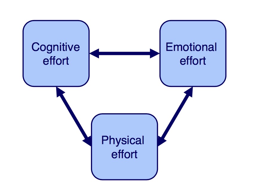
The three components of the conscious system describe the state in which the system is and why it needs to be “controlled”. It requires physical, cognitive and emotional effort to steer and direct the train of thought.

System 2: The unconscious processing machine works with biases, associations, heuristics and is highly parallel. It tries to reduce complex data structures into comprehensible pieces of information that can be analyzed by the conscious stream.

Unfamiliar processes (such as driving a car) can at first require the conscious system to analyze and understand the actions required to perform the tasks. However, the repetitive nature of the activities quickly allow the unconscious system to take over the work.

Heuristics and Biases

Literature: Kahneman & Tversky (1974): Judgment under Uncertainty: Heuristics and Biases, Science, 185(4157), pp. 1124-1131.

Heuristics work by the individual quickly asserting certain structures or patterns based on a limited amount of input data. Often these heuristics are coupled with the need to predict or assert certain characteristics, e.g. a stock price change in the next weeks. There are many automatic rule-sets that most humans follow with their unconscious system which often lead to good results but can also lead to systematic errors.

Representative Heuristics

Choose between A and B, in relation to C. How much is A or B similar to C? The one that is more similar gets chosen. A simple example is “whose kid is this? Dark hair, dark skin, probably Michaels.” This heuristic makes sense in many contexts but can cause issues in others. If one gets a detailed explanation of a persona and then a list of jobs with the task to assign him to the most likely job he will be working in, most people choose the job whose representatives are regarded by culture as similar to the described persona. So a “successful, fit, mathematically interested, technical, adventurous, success driven, academic…” persona when having to select among “cashier, teacher, office clark, astronaut”, most people would choose the last. However, people show an insensitivity to prior probability of outcomes. What are the chances that anyone is an astronaut vs. these other very common jobs? Marginal at most. But people associate these descriptions with astronauts so the described persona is representative of the group and therefore considered most likely.

• people ignore overall probability of a certain situation being true if
• a description / situation is representative of one of the options even if
• the option is far less likely than all others in the base distribution.

insensitivity to sample size

Even professional Psychologists overestmiate the representative value of small sample sizes for a larger corpus. Overall small sample sizes are more likely to exhibit more extreme values on distribution scales.

Misconceptions of chance

The classic case is the gamblers fallacy. Chance doesn’t self correct, it just dilutes over repetition. Therefore after 5 heads at a coin toss, the next toss is still 50:50, no “it must be tails now”.

Insensitivity to predictability

Watch 3 couples for 20 minutes each then predict if they will still be together in 5 years from now: Most people would base their predictions on what they observed. But realistically, one knows nothing about the relationships so all predictions should be the same and all should be the average (whatever that is).

Illusion of validity

People think they are right even though they base their decision on flaky base data. Once they have decided, they stick to their decision with higher confidence than the base information is offering.

Misconceptions of Regression

Generally, there is a regression towards the mean. Although the gamblers fallacy is people expecting this regression, there are also cases in which it is misinterpreted. Let’s imagine students on average achieve a (B-) in school. If a student achieves an A/A+, a teacher will congratulate the student. Yet statistically, the next exam will be more likely to be closer to the average than another good grade again. On the other hand if a student got an F, the teacher will be critical. But statistically, the student will be more likely to get a better grade next time, independent on the criticism or compliments. In both cases, the teacher could in hindsight interpret: “congratulating makes my students write less good exams and criticism fosters good grades”. This would be detrimental to the goals.

Availability bias and examples

Those cases that are easier to recall are usually considered more likely to be true. Examples are

1. Retrievability: The ability to retrieve instances from memory 2) Effectiveness of a search set: Samples of words with r in 1. or 3. letter → 3rd is harder to “search” in the mind, e.g. less likely? false 3) Bias of imaginability: If one cannot imagine something, it is less likely considered to be true

Anchoring and inadequate adjustment

One gets anchored on a number. Examples are:

• Bargaining on a market place in turkey
• Salary discussions and previous salaries

However, even when we are aware of what the anchor is (e.g. an average), we still do not adjust adequately.

Overconfidence, Choices and Frames

Literature:

• Kahneman & Tversky (1979), Prospect theory: An analysis of decision under risk. Econometrica 47(2):263–292.
• Tversky & Kahneman (1992), Advances in prospect theory: Cumulative representation of uncertainty, J. Risk Uncertainty, 5(4):297–323.
• Thaler (1999), Mental Accounting Matters, Journal of Behavioral Decision Making, 12 (3), 183-206.

Prospect theory

2 Stage decision process:

1. Editing: Reference point defined.

• Better → gains
• worse → losses

2. Evaluation of potential outcomes based on function which can be seen as a utility function

• The function is asymmetrical, losses are dreaded more than gains are cherished (loss aversion)
• 50:50 chance of €1000 vs safe 500: ppl choose 500
• same in negative: People prefer risk: Risk seeking in losses, aversion in gains

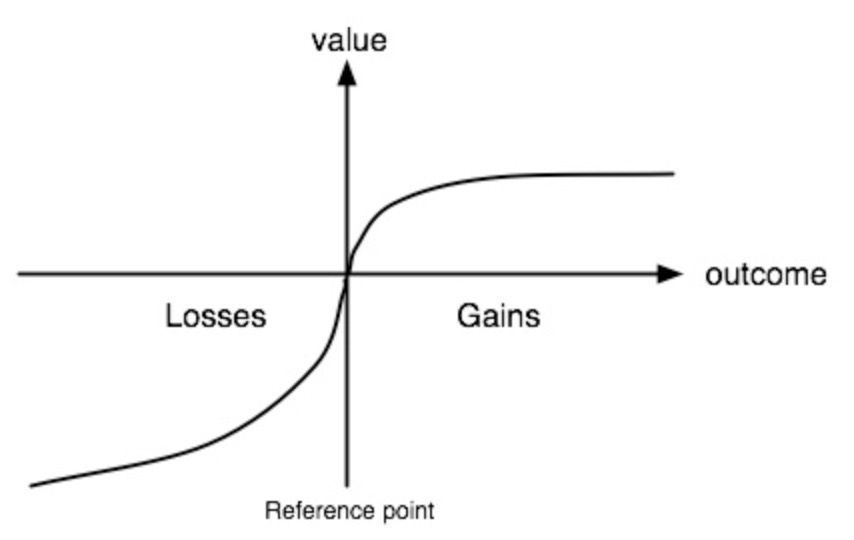
• People are risk-averse in the gains and risk-seeking in the losses

Endowment effect

• Loss aversion discourages trade

• Purchasing party considers products of less value than selling party

• → mugs experiment:

  • What’s the mug worth? 5€. Here it’s yours. What’s the mug worth? 6€

[ WTP < WTA $ ]

Probability weighting function

People tend to overweight small probabilities and underweight large probabilities. E.g. a 3% of getting killed is regarded as a big risk but then the subjective risk does not double from 3 to 6%.

Allais paradox

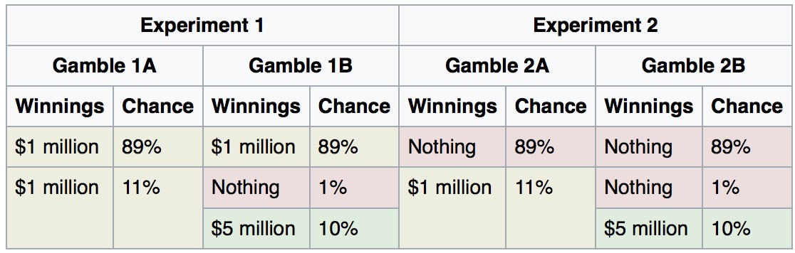
People tend to choose 1A and 2B. But 1A is a “sure thing” while 2B is a gamble.

Framing

Subjective interpretation of alternatives different in different contexts, when explained differently. Humans aren’t capable of extracting the abstract objective value from the displayed offer. E.g.

• credit card surcharge (loss aversion triggers) vs.
• cash discounts

Most people rather forfeit the discount than accept a surcharge.

Hedonic Framing

aka make people feel better about the objectively same situation.

• Segregate gains (winning 3 small things is more lucky than 1 equivalent large thing)
• Integrate losses (loosing once big time is better than often and a little)
• Integrate small losses with large gains
• Segregate small gains from large losses → silver linings

Mental Accounting

You go to the movies. Before the movie theater you loose $10. Do you still go to the movies?

You go to the movies. Before arriving you realize you lost your $10 pre-purchased ticket. You still go?

The Cab drivers example: On bad days, people tend to work long hours to achieve their set target of earnings per day. On busy days many work less time as they reach that goal quicker. Rationally one should work long hours on busy days and quit early on slow days.

Planning fallacy

• Over optimism in planning
• estimates usually too close to best case scenarios
• known-knowns (best-case), known-unknowns (buffer), unknown-unknowns (doors and corners)

Improvement strategies usually include statistics based estimates (scrum velocity) of past observations.

Social preferences

Altruism

Economic altruism vs. Psychological Altruism

• EA: a deed that inflicts material costs on the performing actor in order to increase the material fitness of someone else
  • motivation does not matter, i.e. it can be for reputation or expected later return of the favor
• PA: same cost type as with EA and it is not motivated by psychological advantages
  • So if I give my girlfriend a gift because it makes me happy to see her happy, it is not considered to be altruism.

Outcome-based preferences: Distributive fairness (Inequality aversion)

• Preference for fair outcomes:

  • relative to a standard

• Reciprocity

  • rewarding kind behavior (positive R)
  • punishing negative behavior (negative R)

• Evidence for fairness: There is some evidence based on field research and questionnaires.

• Downside: No concern for process, just looking at outcomes

Social preferences

• If A includes in its utility function the result of the utility of B, it has social preferences
• Are social preferences consistent, rational?
• a substantial percentage of people are inequality averse
  • However they are more inequality averse in the case of being the less well endowed → more envious than feel guilty

Bolton-Ockenfels model

• Individuals include in their utility function $U_i = U_i(x_i, s_i)$ both their received value as well as their “fair share”, having a maximum in $\frac{1}{n}$, i.e. in the perfect share of the total number of people to share with.

Fairness Games

Should be capable of explaning all of them

• Prisoners Dilemma
  • The concept of offering two to-be-convicted criminals to either betray their partner or stay quiet. Rationally, both betray the other to reduce their own sentence. However, if both betray each other the overall sentence is 2 years each instead of 1 if both kept quiet.
• Public Goods Game
  • Subjects secretly choose how many of their private tokens to put into a public pot. The tokens in this pot are multiplied by a factor (greater than one and less than the number of players, N) and this “public good” payoff is evenly divided among players. Each subject also keeps the tokens they do not contribute
  • If everyone gives everything, the result is maximised
  • Game theory suggests that no one puts in anything
  • Real observations show people entering different amounts into the public pot, usually dependent on the multiplication factor
• Ultimatum Game
  • Player A gets money. He has to pass this to player B. If player B accepts his part, A gets to keep his as well. If B refuses his part, A also gets its share taken away again
• Dictator Game
  • Same a ultimatum game but B just receives money without any chance to act upon it
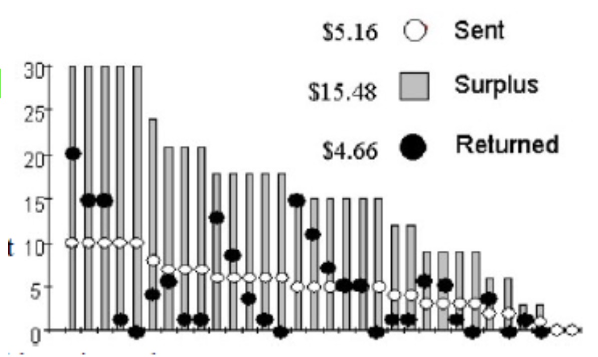
• Trust Game
  • Adaptation of dictator game. A gets money, can send to B and B gets a multiplication of the sum. A hopes/trusts B to send back the invested amount (or more) to A
  • Centipede: Multi-stage trust game
  • Gift exchange: Multi-Player trust game
• Trust and punishment game
  • Adaptation of the trust game. Trustor can impose a fine before sending money to punish trustee if no money is sent back.
    • If fine is available but not imposed, people send more money back. Acknowledgement of trust

Empirical data on fairness games

• Dictator game: 1/3 gives nothing, 1/3 gives half, rest in between
• Ultimatum game: Most give 30-50% with little rate of rejection
  • no one gives more than 50%
  • rejection rate is anti-proportinal to share-rate
• Trust game: On average, players are just compensated their investment → B not valuing the trust received by player A
  • But: only “average” most people either give back more or less, few actually return investment only.
• Trust and punishment game: Similar results have been seen for “fines for picking up your children late”. After introduction of the fine, more people picked them up late as they saw it as a “fair payment” for their late arrival

Intentions-based preferences (Reciprocity)

• Reciprocity: preference to repay received treatment with similar treatment in the future.

Trust and Social Identity

• Behavior towards strangers vs. friends / family in the trust fairness games. Ingroup vs. Outgroup effects are proven

Behavioral Forecasting

Setting

General Approach

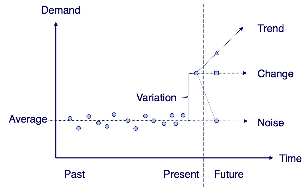
Kremer et al.: How do subjects detect a change of demand level

Time-Series Modeling − Forecast Modeling

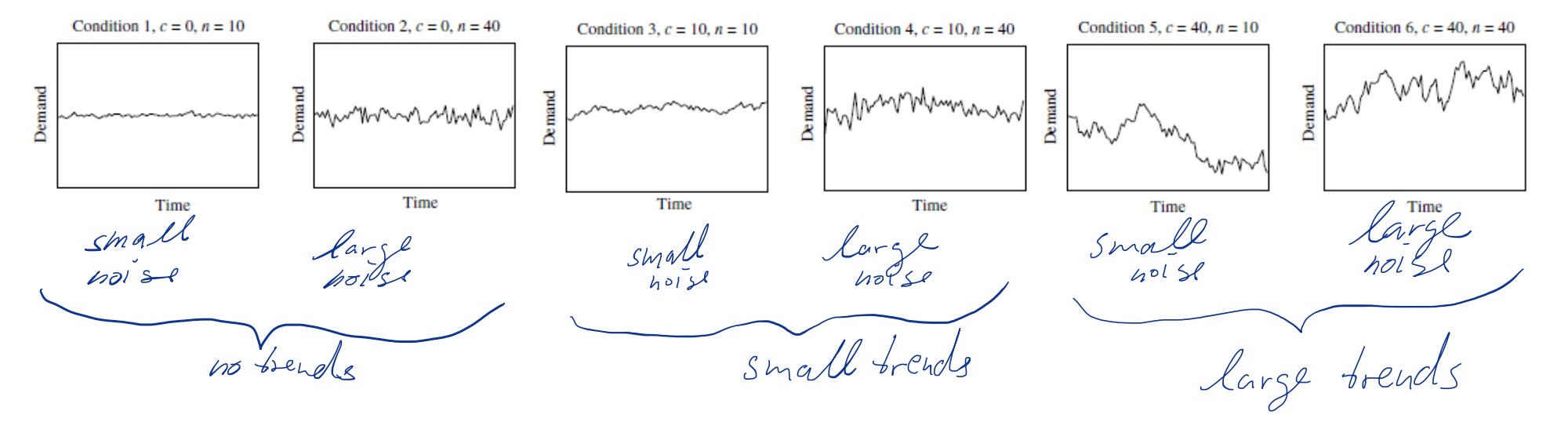
• model idea: Temporary shocks and permanent trends

Single exponential smoothing in time-series modeling

• Forecast formula: $F_{t+1} = \alpha D_t + (1 - \alpha)F_t = F_t + \alpha(D_t - F_t)$

  • $D_t$ describes the demand in t

• optimal $\alpha$ expressed through change-to-noise ratio $W = \frac{c^2}{n^2}$

• $a^*(W) = \frac{2}{a+\sqrt{1+ 4\div w}}$

  • optimal $\alpha$
  • large c → small sqrt → small dividend → large ɑ
  • larger $W$ → more weight on recent demand figures

Experiment

Hypothesis: Humans overreact on changes that are rationally likely caused by noise and underestimate real trends

• Actual experiment demand is statistically random with no long-term trends in place
• performance deteriorates with increasing noise and change
  • 37% imagine trend where it is not one 42% act rationally
• Forecase performance is negatively influenced by
  • systematic decision biases
  • random errors

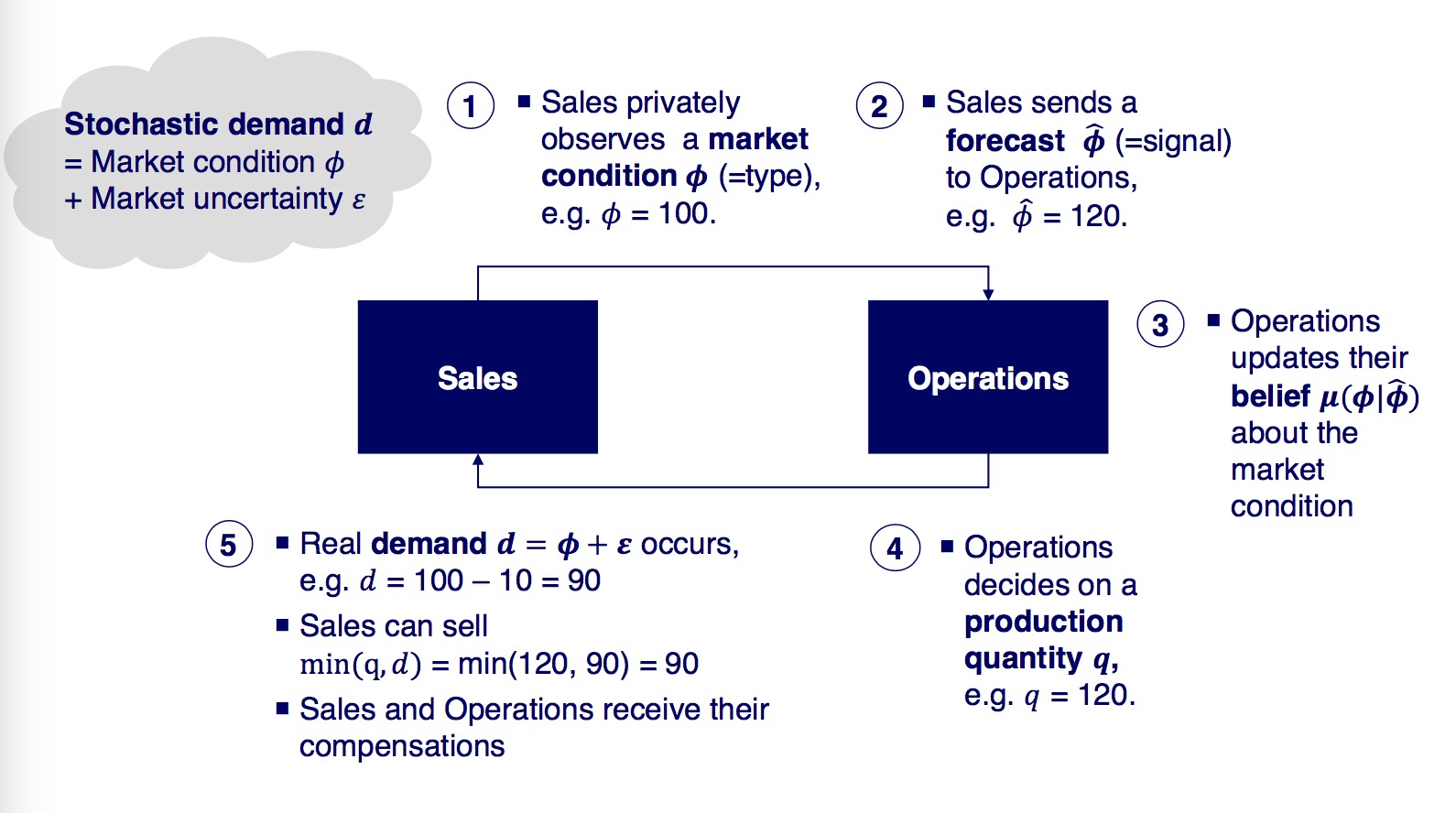
Trust in Forecast Information Sharing

• Manufacturers need credible forecasting information from their retailers
  • if the forecasts do not match real world expectations, large over/underproductions are the result

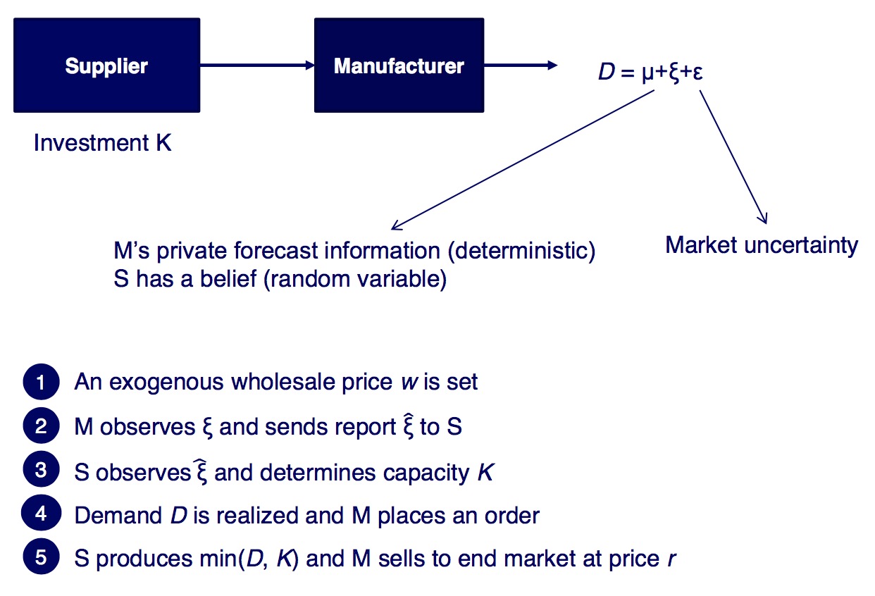
If the forwarded demand forecast $\hat{\xi}$ is not realistic (i.e. too large), the retailer minimizes his risk of incurring underage costs at the cost of expectable overage costs for the manufacturer.

• sending $\hat{\xi}$ is costless, non-binding and called cheap-talk

Empirical data on forecast information sharing

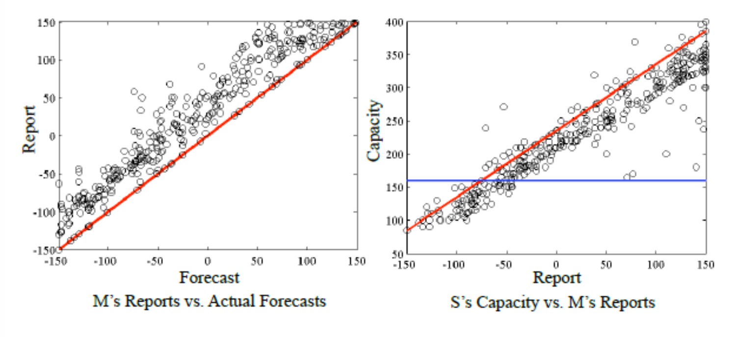
• retailers systematically overreport demand
• Manufacturers systematically discount forecasts by retailers
• result → non optimal supply chain but some correction automatically in place

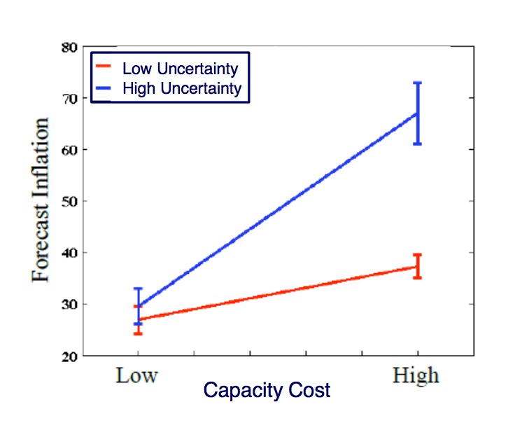
• low capacity cost reduces forecast inflation

• lowering uncertainty mediates inflation in high capacity cost environments

• Perfect Bayesian Equilibrium is uninformative

  • comes from game theory: A talks shit B doesn’t believe him.

• including trust in the model corrects the inflated reports adequately

• Managerial Insights:

  • complex and highly variable products: trust or strict contracts required
  • simple products: wholesale price + cheap talk is fine, inflation less likely

Implications for Behavioral OM & Design of Experiment

Within subjects	Between subjects
✅ easier significances	✅ no order effects
❌ order effects	❌ larger samples necessary
	❌ individual effects hard to extract

One-shot games	Repeated game
no strategic spillovers	learning
easy	more observations
	convergence to Equilibrium

Parter Design	Stranger Design
item of observation is team, stays continuous	item is still group but it is changed all the time
Both offer good observations. If one wants to observe interaction within a team over time, partner design is necessary. Both however include social preferences and other sociological biases

• role switching: subjects learn game from all angles
  • might lead to information losses
  • can be overly simplified as subject understands lower level dynamics of the (simplified) game → model not close enough to reality anymore

Behavioral Contracting

Research Papers for Behavioral Economics

Decision Bias in the Newsvendor Problem with a Known Demand Distribution

Authors: (Schweitzer, Cachon 2000)

• $q_n$: Optimal risk-neutral order quantity

Question: Why do decisions deviate from profit maximisation?

• risk-averse behavior
• prospect theory applies: retailers risk high potential losses instead of accepting continuous small losses

Types of decision makers

• risk neutral: $q_t = q_n \forall \text{rounds} t$
  • utility = expected profit
• risk averse and risk seeking: classic concave/convex curves
• prospect theory aligned:
  • if only gains are possible: under-ordering
  • if only losses are possible: over-ordering
• waste-averse: A Decision maker dislikes salvaging excess Inventory
  • avoids over-ordering
  • $q_t \leq q_n$
• stockout-averse: Dislikes loosing potential sales
  • $q_t \geq q_n$
• underestimated opportunity costs
  • underestimates value of foregone sales
  • similar to waste-averse, but different motivation.
• minimizing ex-post inventory error
  • $q_t \leq q_n$ for high profit products
  • $q_t \geq q_n$ for low profit products
  • irrational: High profit products are worth over-ordering as few sales can compensate several unsold orders
  • probably due to anchoring to mean demand

Experiment and results

• 34 subjects (MBA OM) [quiet unrepresentative…]
• demand distribution is known-known
• no change in order sizes over time

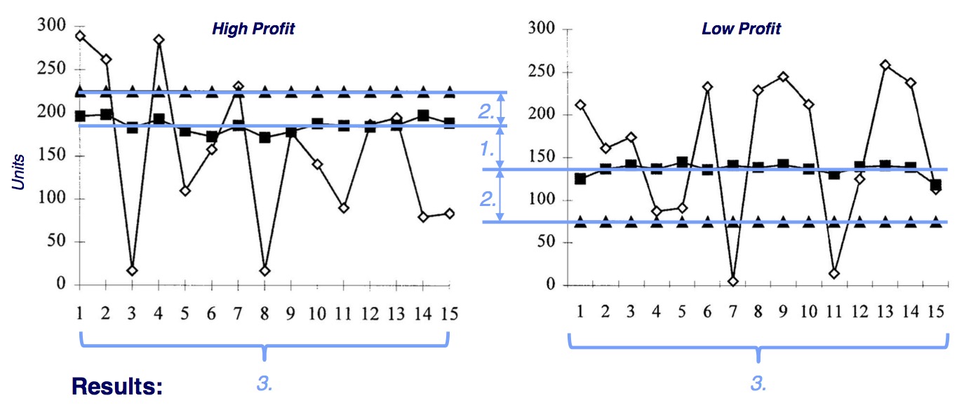
• people order too few for high profit and too many for low profit.
• people do not learn. Behavioral explanations such as risk aversion, risk-seeking, waste aversion, … insufficient
• guessed reason: anchoring, insufficient rational reprocessing of information given
• experiment repeated with high demand environment: Same results, no change in demand in DLOW/DHIGH

Managers and Students as Newsvendors

Autors: Bolton, Ockenfels, Thonemann. (2012)

University of Cologne seems to be big in this field. Or we just read their stuff because we are from the same University

A comparison study that shows the different behaviors of managers and students when taught a certain demand distribution and then asked to perform experimental ordering in the newsvendor model. No significant differences were found?

Reference Dependence on Multilocation Newsvendor Models: A Structural Analysis

Authors: Ho, Lim, Cui 2010

• Centralized vs. decentralized newsvendor decision makers
• People dislike supply/demand mismatch 6-10 times more than they like money

Setting: Cheap-talk forecast communication under asymmetric forecast information

• supplier
  • needs to invest in capacity
  • has “cheap talk” as input
  • somewhat relies on forecast of manufacturer
• manufacturer
  • has better market information
  • has incentive to inflate forecast to ensure capacity of supplier

Trust in forecast sharing for repeated interactions

• lower forecast inflation
• higher capacity
• higher efficiency

An explanation can be the fact that the parties will still have to rely on each other in the future and therefore are more willing to provide correct forecasts to ensure continued cooperation is possible.

Approaches towards ensuring proper forecast sharing

• advance purchase contracts (risk sharing)
• forecast error penalty contracts (risk sharing)
• penalty mechanisms for repeated interactions

Designing Incentive Schemes for Truthful Demand Information sharing

The goal is to compare different incentive systems for sales departments

• Sales-Bonus-only: forecast error not penalized
• Absolute forecast error: deviation of forecast from demand penalized
• differentiated forecast error: over-forecasting penalized harder

Since sales and operations usually interact with one another, the operations utility function is also modelled. However it is kept simple with loss-aversion being the only factor in the utility model.

Results? None described

Learning by Doing in the Newsvendor Problem

Authors: Gary E. Bolton, Elena Katok

• experience improves performance
• restricting ordering to standing orders of 10 ordering rounds improves performance
  • keeps decision makers from chasing demand and

In the context of the newsvendor model, people have been shown not to behave rationally. This paper seeks to find organizational features that promote optimal behavior.

Previous Research has shown decision makers to show many biases such as the anchoring bias.

The authors performed 3 experiments:

1. an extended experience with 100 rounds as opposed to 30 rounds in previous research.
2. forward-looking learning investigation: They provide the participants with tracking information on forgone and taken decisions to show missed profits and realized profits
3. Investigating small-numbers bias: Forcing participants to make standing orders for 10 rounds at a time instead of for each round.

The authors find increased experience to help finding the optimal order point. However the Improvements are smaller than they should be. They found additional information about forgone profits to not lead to significant improvements. Lastly, making the participants enter standing orders of 10 rounds each significantly improves the performance. Generally, newsvendors do better in high-safety-stock conditions than in low ones.

A conclusion for organizations is the inhibiting of inappropriate responses to short-term information. This leads to decision makers not letting themselves react to short-term spikes and drops and rather act on a more continuous pattern.

Designing Pricing Contracts for Boundedly Rational Customers: Does the Framing of the Fixed Fee Matter?

	Fixed fee not charged	Fixed fee charged
$	p	= 1$
$	p	\gt 1$

• two part tariff(TPT): significant coordination expected
• three part tariff: no coordination improvements over two p expected
• block tariff: Expecting loss aversion effects based on the idea of mental accounting / prospect theory
  • losses and gains are segregated → hedonic framing

Fixed fee	integrated costs
$qw + F$	$q(\frac{F}{q} + w)$
$qw + F \leftrightarrow q(\frac{F}{q} + w)$

Obviously, the two contracts are of equivalent mathematical value. However, the fixed fee is considered an “extra cost” and triggers loss aversion. In a mathematical sense, the manufacturer would sell his items at retail price $w=c$, assuming both $c, p$ are common knowledge in the supply chain. He would then correct this lack of profit by setting a fixed fee $F = \frac{d*c}{2}$, so half the total profit of the overall supply chain profit. This would, theoretically, lead to the retailer ordering an optimal amount and giving half of its expected profit to the supplier.

Results

The optimal channel efficiency ($\epsilon$) was never reached. The two-part tariffs actually performed worse than the linear-price contracts (LP) in the overall average. The quantity discount (QT) did improve channel efficiency. It is interesting however, that for if the retailer accepted (A) the contract, the channel efficiency was much higher for both coordinating contracts, that is, the supply chain was successfully coordinated, if the retailer accepted the contracting terms.

$\epsilon(LP) = 72.95$ $\epsilon(TPT) = 69.51$ $\epsilon(QD) = 76.37$ $\epsilon(LP \mid A) = 77.85$ $\epsilon(LP \mid TPT) = 93.62$

It clearly shows, once the retailer accepts the contract, TPT is much more successful at coordinating the supply chain. The authors also showed that compressing the fix payment, that is hiding the fix payment in the wholesale price, reduces the loss aversion and improves channel coordination.

They also tested for fairness by changing the suppliers payout rate for the real-world payments but kept the retailers rate the same. As such, for each hypothetical dollar, the supplier earned more money than the retailer. However, this did not change the acceptance rate of the contracts offered which the authors interpret as fairness not being a factor in the decision process of the retailer.

Contracting in Supply Chains: A Laboratory investigation

Authors: Katok, Wu (2009)

• Comparing 3 contracting schemes: Wholesale, buyback and revenue sharing
  • buyback and revenue sharing are mathematically equivalent but it is shown that they are not seen as such by subjects
• low/high risk environments lead subjects to prefer one of the two risk-sharing contracts over the other
• learning mediates the effects of irrational behavior
• player playing both sides, both times against/with an algorithm
  • approach novel as it removes social preferences

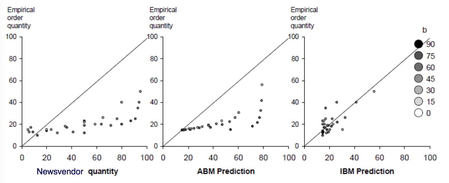
Designing Buyback Contracts for Irrational But Predictable Newsvendors

Authors: Becker-Peth, Katok, Thonemann (2013)

• Research Question: How to get contracts designed in a way that the subjects consider behave optimally, i.e. they are coordinating the supply chain

To get a better model, the authors include anchoring, loss aversion and mental accounting $\alpha, \beta$ and $\gamma$ in the model. They apply this both to the overall corpus of the subjects as well as calculate these variables for each individual to create a individual-based model. They then construct contracts that the model predicts will be more effective with the subjects while also coordinating the supply chain.

Social Preferences and Supply Chain Performance: An Experimental Study

Authors: Loch Wu - 2008

• State of research at point of writing:
  • Before Katok, Wu → social preferences effects unknown, most divergence of theoretical performance of contracts and practical performance is attributed to individual behavioral attributes.
  • social preferences known from behavioral psychology → transferring concepts to behavioral economics

Experiment

The experiment is structured into 3 different conditions: Control, Relationship and Status. The control group is neutrally treated, the relationship group are pairs of 2 that are being introduced to each other before beginning the experiment and the status group is confronted with each others total profit after each round to spur competition.

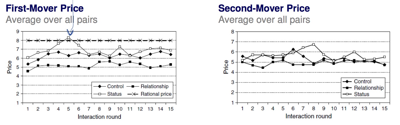
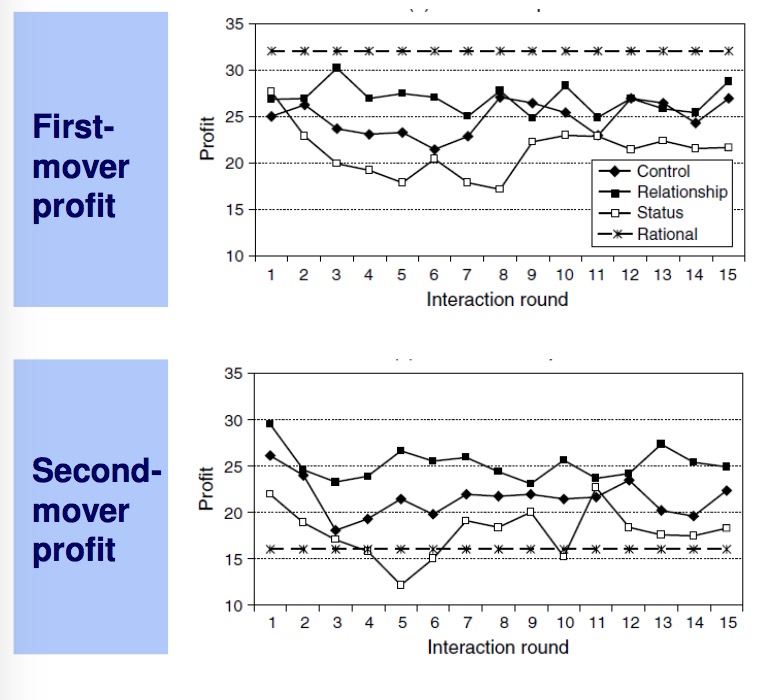
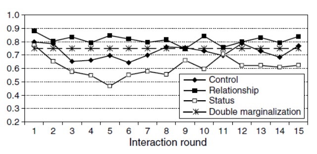
It becomes clear that the relationship treatment is performing much better than the status treatment. Also, the bump in the first-mover graph shows the reaction of the supplier to its lowering profits and also the realization that he is taking an overproportional part of the margin.

• social preferences have an impact
• pricing is more aggressive in a status context
• second mover increases prices when first mover increases prices → economically irrational as it reduces overall profits

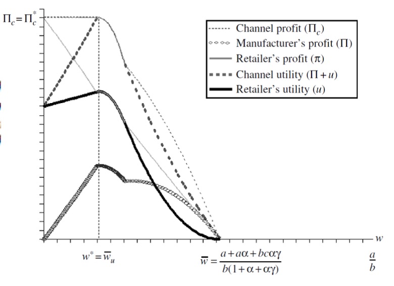
Fairness and Channel Coordination

Authors: Cui, Zhang - 2007

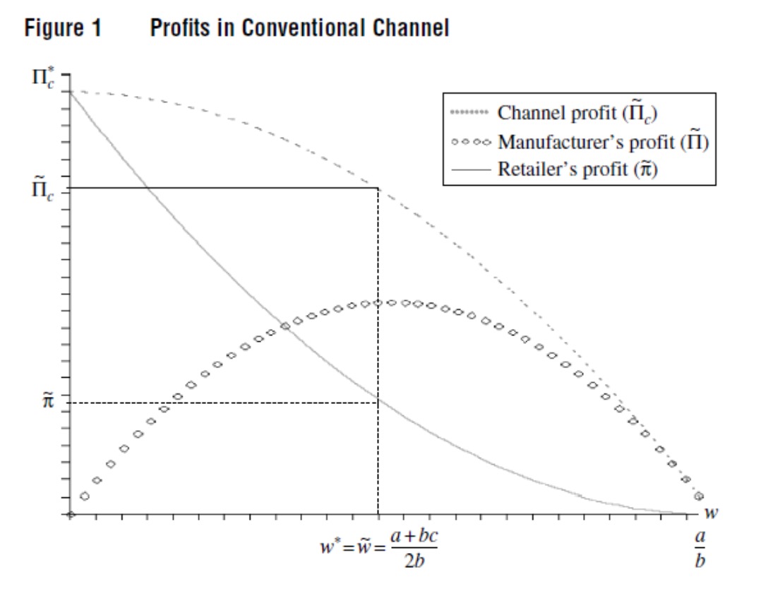
• the manufacturer is responsible for enabling a coordinated supply chain by offering a $w$ that leads the retailer to purchasing an amount $q$ that is optimal in relation to the demand $d$

Appendix

Variables (v1)

Variable	description	environments
$q$	Order Quantity	newsvendor
$w$	wholesale price per item	wholesale contract

Names+Years

• Bolton & Ockenfels - 2000: Motivated by their payoff standing in relation to other people, i.e. the fairness of their payoff. People feel more envious than guilty
• Behavioral Forecasting
  • Özer, Zheng, Chen - 2011
  • Kremer, Minner, Van Wassenhove - 2010
• Behavioral Inventory
  • Schweitzer and Cachon - 2000
  • Bolton, Katok - 2008
  • Bolton Ockenfels, Thonemann - 2008
  • Ho, Lim, Cui - 2010
• Behavioral Contracting
  • Becker-Peth, Katok, Thonemann - 2013: How to construct buyback contracts optimally under the influence of the three variables: anchoring, loss aversion and TODO
  • Katok, Wu - 2009
  • Cui, Raju, Zhang - 2007
  • Loch, Wu - 2008
  • Ho, Zhang - 2008

Vocabulary / Terminology

• Newsvendor Model
• Order rationioning: manufacturer forecasts demand and produces according to his own expected demand. If demand is higher than production quantity, each retailer gets a proportionally reduced amount.
• Order batching: Coordinating multiple retailers by the manufacturer → setting delivery dates so that the overal output is continuous. Compare Barilla case
• Postponement: Move customization of products for different markets at end of supply chain to avoid complex supply chain structures
• Component commonality:idea of using standard parts that cost more per piece but reduce complexity. There is a point of equilibrium which equals out the savings in complexity costs for supporting many different variants vs. the increase in unit cost.
• Continuous Review Inventory Model
• Backorder level: The number of backorders and days where people need to wait. It doesn’t only capture the times when a order cannot be filled but also the time an order has to wait before it gets filled. Can be simulated by having a non-filled order re-request a product in each period until it is being served
• Economic Order Quantity Model
• Periodic Review Inventory Model
• Service Levels
• Availability and representativeness in Forecasting
• Anchoring in Inventory decisions
• Bounded Rationality
• Decision Support
• Framing of decisions
• Reference Points
• Mental Accounting
• treatment: particular condition of an experiment. Main/control treatment, different variations with adapted parameters, …
• Priming
• Risk- loss preferences
• Prospect Theory
• Probability perception
• The Wilcoxon signed-rank test is a non-parametric statistical hypothesis test used when comparing two related samples, matched samples, or repeated measurements on a single sample to assess whether their population mean ranks differ (i.e. it is a paired difference test).
  • It can be used as an alternative to the paired Student’s t-test, t-test for matched pairs, or the t-test for dependent samples when the population cannot be assumed to be normally distributed.
  • A Wilcoxon signed-rank test is a nonparametric test that can be used to determine whether two dependent samples were selected from populations having the same distribution.
• The Wilcoxon-Mann-Whitney Test is a nonparametric test of the null hypothesis that it is equally likely that a randomly selected value from one sample will be less than or greater than a randomly selected value from a second sample.
  • Unlike the t-test it does not require the assumption of normal distributions. It is nearly as efficient as the t-test on normal distributions.
  • A Wilcoxon signed-rank test is a nonparametric test that can be used to determine whether two dependent samples were selected from populations having the same distribution.
• Double marginalization: The effect of two distinct decision makers trying to optimize their individual margins without regarding the fact that their decisions also effect the other decision makers decision.